Stress Tensor

Stress Vector

Most readers are already familiar with the well-known cube that illustrates the stress components. However, this cube is not a physical block of material extracted from the body; rather, it is a convenient representation of the stress field at a point, depicted using three mutually perpendicular planes defined by the base vectors (e1, e2, e3).

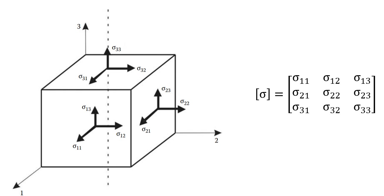
Ref: Khennane A., Introduction to Finite Element Analysis Using Matlab and Abaqus

Due to static equilibrium conditions and the absence of body torques, the stress tensor is both real-symmetric. This symmetry ensures that the moments acting on an infinitesimal element are balanced. \[\sigma_{ij} = \sigma_{ji}\]

According to Cauchy’s stress theorem, if the stress tensor field at a point is known, its stress vector in a plane defined by normal vector {n} can be calculated with the projection of tensor field on the plane.

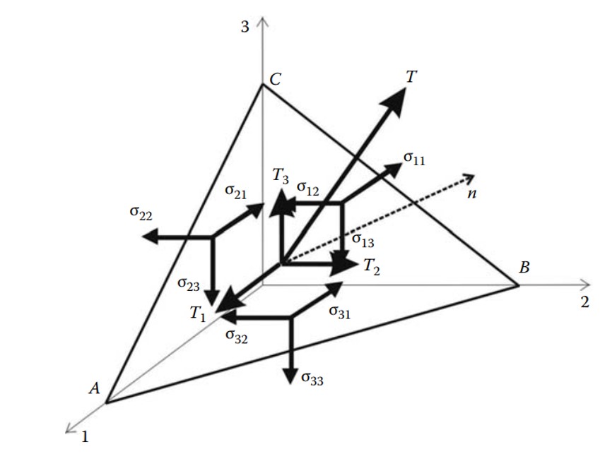
Ref: Khennane A., Introduction to Finite Element Analysis Using Matlab and Abaqus

The stress vector on a cross-section is referred to as the traction vector, {T}. It is defined as the force vector acting on a cross-section divided by the area. The traction vector generally has both normal and tangential components with respect to the plane; in other words, it is not necessarily aligned with the normal vector. \[\{T\} = [\sigma]^T \{n\} = [\sigma] \{n\}\]

Principal Stress

It is possible to select a plane where the traction vector is parallel to the surface normal, meaning that only normal stresses act on the plane. This condition is described by the following relationship: \[\{T\} = [\sigma] \{n\} = \lambda \{n\}\]

This is an eigenvalue problem. Since the stress tensor is real and symmetric, it has real eigenvalues and orthogonal eigenvectors. To express the solution, two matrices can be defined:

• [V]: a matrix whose columns are the eigenvectors
• [Λ]: a diagonal matrix containing the eigenvalues

The eigenvectors indicate the principal directions, while the eigenvalues represent the principal stresses. In the principal basis, the stress tensor is diagonal and represents pure normal stresses without any shear components. \[[V] = \begin{bmatrix} \{v_1\} \\ \{v_2\} \\ \{v_3\} \end{bmatrix}, \quad [\Lambda] = \begin{bmatrix} \sigma_1 & 0 & 0 \\ 0 & \sigma_2 & 0 \\ 0 & 0 & \sigma_3 \end{bmatrix}\]

Orthogonality of Eigenvectors

It is worth emphasizing the orthogonality of the eigenvectors of real-symmetric matrices, as this property is fundamental to many other applications, such as modal analysis and mode superposition. In fact, finite element analysts frequently work with real-symmetric mass and stiffness matrices that exhibit the same behavior.

Consider two eigenvectors of the stress tensor: \[[\sigma] \{v_1\} = \lambda_1 \{v_1\} \\ [\sigma] \{v_2\} = \lambda_2 \{v_2\}\]

Taking the dot product of the second eigenvector with the first equation: \[\{v_2\}^T [\sigma] \{v_1\} = \lambda_1 \{v_2\}^T \{v_1\}\]

Since [σ] is symmetric: \[([\sigma] \{v_2\})^T \{v_1\} = \lambda_1 \{v_2\}^T \{v_1\}\]

Substituting from the second eigenvalue equation: \[(\lambda_2 \{v_2\})^T \{v_1\} = \lambda_1 \{v_2\}^T \{v_1\}\]

Since eigenvalues are distinct, the only solution is: \[\{v_2\}^T \{v_1\} = 0\]

This shows that the two eigenvectors must be orthogonal. In matrix form, this orthogonality condition is written as: \[[V]^T [V] = [I]\]

This also implies that the transpose of the orthogonal matrix is equal to its inverse: \[[V]^T = [V]^{-1}\]

All eigenvalues and eigenvectors can be expressed simultaneously in the following matrix equation: \[[\sigma][V] = [V][\Lambda]\]

Which also requires: \[[V]^T [\sigma] [V] = [\Lambda]\]

This equation represents the transformation of the stress tensor into the eigenbasis (principal basis). Conversely, transforming back to the standard coordinate basis: \[[V] [\Lambda] [V]^T = [\sigma]\]

Eigenvector matrix [V] acts as a transformation matrix from eigenbasis to standard coordinate basis, while its transpose performs the reverse transformation. This eigenbasis transformation is a special case of the more general coordinate basis transformation. Mode superposition is an application of this same concept to multidimensional dynamic systems.

Coordinate Transformation

Let us assume that the standard basis vectors are {e1, e2, e3} and we want to express vectors and tensors in another coordinate system defined by {e1’, e2’, e3’}. The rotation matrix between these two bases is defined by using directional cosines between unit vectors as shown in [Q]. Alternatively, a sequence of rotations about yaw, pitch, and roll axes can also be used to define a general 3D rotation. Rotation matrices are orthogonal. \[[Q] = \begin{bmatrix} \cos(e_1', e_1) & \cos(e_1', e_2) & \cos(e_1', e_3) \\ \cos(e_2', e_1) & \cos(e_2', e_2) & \cos(e_2', e_3) \\ \cos(e_3', e_1) & \cos(e_3', e_2) & \cos(e_3', e_3) \end{bmatrix}\]

In Cartesian coordinates, the standard basis [E] is simply the identity matrix: \[[E] = \begin{bmatrix} 1 & 0 & 0 \\ 0 & 1 & 0 \\ 0 & 0 & 1 \end{bmatrix}\]

Unit vectors of transformed basis can be arranged in matrix form as: \[[E'] = \begin{bmatrix} (e_1)'_x & (e_2)'_x & (e_3)'_x \\ (e_1)'_y & (e_2)'_y & (e_3)'_y \\ (e_1)'_z & (e_2)'_z & (e_3)'_z \end{bmatrix}\]

Transformation matrix can also be expressed using these unit vectors: \[[Q] = [E']^T = \begin{bmatrix} (e_1)'_x & (e_1)'_y & (e_1)'_z \\ (e_2)'_x & (e_2)'_y & (e_2)'_z \\ (e_3)'_x & (e_3)'_y & (e_3)'_z \end{bmatrix}\]

Now, consider a vector {u} defined in the standard coordinate system. Its representation in the new coordinate system is: \[{u'} = [Q]{u} = [E']^T {u}\]

The transformation of a second-order tensor, such as the stress tensor, into the new coordinate system is given by: \[[\sigma'] = [Q][\sigma][Q]^T = [E']^T [\sigma] [E']\]

This is the same equation used during transformation into the eigenbasis.

Stress Invariants

The characteristic equation of the tensor is used in the solution of eigenvalue problem. \[\sigma^3 - I_1 \sigma^2 + I_2 \sigma - I_3 = 0\]

The invariants of the stress tensor in index notation are defined as follows: \[I_1 = \sigma_{ii}\] \[I_2 = \frac{1}{2} \left( \sigma_{ii} \sigma_{jj} - \sigma_{ij} \sigma_{ji} \right)\] \[I_3 = \text{det}([\sigma])\]

Stress invariants are invariant under a change of coordinate basis. They can also be computed using the principal stresses: \[I_1 = \sigma_1 + \sigma_2 + \sigma_3\] \[I_2 = \sigma_1 \sigma_2 + \sigma_2 \sigma_3 + \sigma_3 \sigma_1\] \[I_3 = \sigma_1 \sigma_2 \sigma_3\]

I1 is related to hydrostatic stress. A key property of I1 is: \[I_1 = \sigma_1 + \sigma_2 + \sigma_3 = \sigma_{11} + \sigma_{22} + \sigma_{33}\]

On the other hand, I2 is associated with the deviatoric part of the stress tensor. The hydrostatic stress tensor represents a mean stress that tends to change the volume of the stressed body, while the stress deviator tensor contributes to the distortion (shearing) of the body.

Deviatoric Stress

The deviatoric stress tensor is obtained by removing the mean hydrostatic stress from the stress tensor. It represents the pure shear behavior of a stress field. \[[S] = \begin{bmatrix} \sigma_{11} & \sigma_{12} & \sigma_{13} \\ \sigma_{21} & \sigma_{22} & \sigma_{23} \\ \sigma_{31} & \sigma_{32} & \sigma_{33} \end{bmatrix} - \begin{bmatrix} \frac{I_1}{3} & 0 & 0 \\ 0 & \frac{I_1}{3} & 0 \\ 0 & 0 & \frac{I_1}{3} \end{bmatrix}\]

The invariants of the deviatoric stress tensor [S] are: \[J_1 = 0\] \[J_2 = \frac{1}{2} \left( s_{ij} s_{ji} \right)\] \[J_3 = \text{det}([S])\]

Von Misses Equivalent Stress

J2 is particularly important because it is used in the definition of Von Misses equivalent stress, which is a scalar value of stress that can be computed from the stress tensor. The Von Mises Yield Criterion, also known as the J2 Yield Criterion, states that a material begins to yield when the von Mises stress reaches the material’s yield strength. It is used to relate a general stress field to the material data obtained from uniaxial tensile tests.

The expression for J2 in terms of the standard stress components is: \[J_2 = \frac{1}{6} \left[ (\sigma_{11} - \sigma_{22})^2 + (\sigma_{22} - \sigma_{33})^2 + (\sigma_{11} - \sigma_{33})^2 \right] + \sigma_{12}^2 + \sigma_{23}^2 + \sigma_{13}^2\]

In terms of the principal stresses, J2 can be written as: \[J_2 = \frac{1}{6} \left[ (\sigma_1 - \sigma_2)^2 + (\sigma_2 - \sigma_3)^2 + (\sigma_1 - \sigma_3)^2 \right]\]

Finally, the von Misses Equivalent Stress is: \[\sigma_{VM} = \sqrt{3 J_2}\]

Alternatively, in terms of the stress components: \[\sigma_{VM} = \sqrt{\frac{1}{2} \left[ (\sigma_{11} - \sigma_{22})^2 + (\sigma_{22} - \sigma_{33})^2 + (\sigma_{11} - \sigma_{33})^2 \right] + 3 \left( \sigma_{12}^2 + \sigma_{23}^2 + \sigma_{13}^2 \right)}\]

In terms of the principal stresses: \[\sigma_{VM} = \sqrt{\frac{1}{2} \left[ (\sigma_1 - \sigma_2)^2 + (\sigma_2 - \sigma_3)^2 + (\sigma_1 - \sigma_3)^2 \right]}\]

An important observation can be made by comparing the conditions of pure uniaxial tension and shear. For these conditions: \[\sigma_{VM_{\text{tension}}} = \sigma_{11}\] \[\sigma_{VM_{\text{shear}}} = \sqrt{3} \sigma_{12}\]

When the same magnitude of stress is applied in both conditions, the shear specimen will yield earlier. The ratio of the yield strengths of the material under these two load conditions is: \[\frac{F_{\text{tension}}}{F_{\text{shear}}} = \sqrt{3} = 0.577\]

This indicates that a material can carry nearly half the shear load compared to the tension load before yielding. A comparison of material tests using different yield criteria is shown in the graph below.

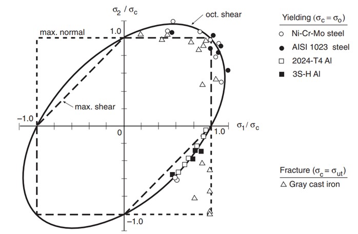Ref: Dowling, N.E., Mechanical Behavior of Materials

Example Calculations

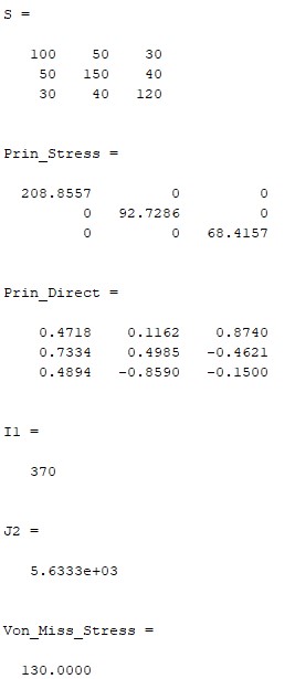
Below is an example of a MATLAB/Octave code that performs the necessary calculations for Von Mises stress and the invariants of the stress tensor.

clc
%define a stress tensor
S=[100 50 30; 50 150 40; 30 40 120]

%calculate principal stresses and directions
[V,L]=eig(S);
%sort eigenvalues
B=diag(L);
[C,I] = sort(B,'descend');
Prin_Stress=diag(C)
Prin_Direct=V(:,I)

%calculate I1
I1=sum(diag(L))

%Calculate J2
J2=1/6*((L(1,1)-L(2,2))^2+(L(2,2)-L(3,3))^2+(L(1,1)-L(3,3))^2)

%Calculate Von Misses Stress
Von_Miss_Stress=sqrt(3*J2)

The output of the code would be: