Maximum Shear Stress
Mohr's Circle
In our previous post about Stress Tensor, it was demonstrated that when the stress field is represented using a tensor, the normal and shear stresses on any plane—defined by a normal vector—can be determined. It was also shown that there exist specific directions in which stress becomes purely normal (tensile or compressive); these are known as the principal stress directions. Additionally, it is possible to identify the planes on which the maximum shear stresses occur.
Mohr’s circle provides a two-dimensional graphical representation of the transformation laws for the Cauchy stress tensor. It allows the graphical determination of the stress components acting on a rotated plane passing through the same point. The mathematical derivation of Mohr’s circle and the equations involved are beyond the scope of this post and will not be discussed in detail here.
Mohr’s circle consists of three individual circles, each corresponding to a rotation about one of the principal directions. A key result from this representation is that the maximum shear stress occurs on planes oriented at 45 degrees to the principal stress planes.
The MATLAB/Octave code provided below can be followed step by step to perform the necessary calculations. The code visualizes the normal and traction vectors, the coordinate axes of both the standard and principal bases, a unit tensor cube, and the cross-sectional plane.
Consider the following stress tensor: \[[\sigma] = \begin{bmatrix} 100 & 50 & 30 \\ 50 & 150 & 40 \\ 30 & 40 & 120 \end{bmatrix}\] Code: Principal Stress Directions
%INPUTS....................................................................
% This code visualizes the traction vector and principal directions of a
% stress tensor. It calculates the normal and shear stresses on a plane.
%..........................................................................
%INPUTS....................................................................
S=[100 50 30; 50 150 40; 30 40 120];           %tensor in standard basis
%S=[208.8557 0 0; 0 92.7286  0; 0 0 68.4157];  %tensor in principal basis
n=[1 0 0]';
%..........................................................................
%..........................................................................
%#ok<*NOPTS>

%calculate traction vector-------------------------------------------------
n=n/norm(n); %convert the normal vector to unit vector
T=S*n;
f1=figure;
figure(f1)
plot3([0 T(1,1)/norm(T)],[0 T(2,1)/norm(T)],[0 T(3,1)/norm(T)],...
    "k","LineWidth",2)
hold on
text(1.15*T(1,1)/norm(T),1.15*T(2,1)/norm(T),1.15*T(3,1)/norm(T),...
    'T','FontSize',14,'color', 'k','FontWeight', 'bold')
%--------------------------------------------------------------------------

%calculate normal ans shear stress on the plane----------------------------
S_normal=T'*n
S_shear=sqrt(norm(T)^2-S_normal^2)
%--------------------------------------------------------------------------

%calculate and plot principal directions-----------------------------------
[V,L]=eig(S);%calculate principal stresses and directions
B=diag(L);
[C,I] = sort(B,'descend');%sort eigenvalues
Prin_Stress=diag(C)
Prin_Direct=V(:,I)
V=Prin_Direct;
plot3([0 V(1,1)],[0 V(2,1)],[0 V(3,1)],"--m","LineWidth",2)
plot3([0 V(1,2)],[0 V(2,2)],[0 V(3,2)],"--m","LineWidth",2)
plot3([0 V(1,3)],[0 V(2,3)],[0 V(3,3)],"--m","LineWidth",2)
text(1.2*V(1,1),1.2*V(2,1),1.2*V(3,1),...
    'P1','FontSize',14,'color', 'm','FontWeight', 'bold')
text(1.2*V(1,2),1.2*V(2,2),1.2*V(3,2),...
    'P5','FontSize',14,'color', 'm','FontWeight', 'bold')
text(1.2*V(1,3),1.2*V(2,3),1.2*V(3,3),...
    'P3','FontSize',14,'color', 'm','FontWeight', 'bold')
%--------------------------------------------------------------------------
The traction vector acting on a plane defined by the normal vector {n} can be calculated as follows: \[\mathbf{T} = [\sigma]^T \mathbf{n} = [\sigma] \mathbf{n}\]
The principal stresses can be determined by solving the eigenvalue problem of the stress tensor: \[\mathbf{T} = [\sigma] \mathbf{n} = \lambda \mathbf{n}\]
The matrix [V] contains the eigenvectors as its columns, while [Λ] is a diagonal matrix composed of the corresponding eigenvalues. The eigenvectors define the principal directions, and the eigenvalues represent the principal stresses. \[[V] = \begin{bmatrix} v_1 \\ v_2 \\ v_3 \end{bmatrix} , \quad [\Lambda] = \begin{bmatrix} \sigma_1 & 0 & 0 \\ 0 & \sigma_2 & 0 \\ 0 & 0 & \sigma_3 \end{bmatrix}\]
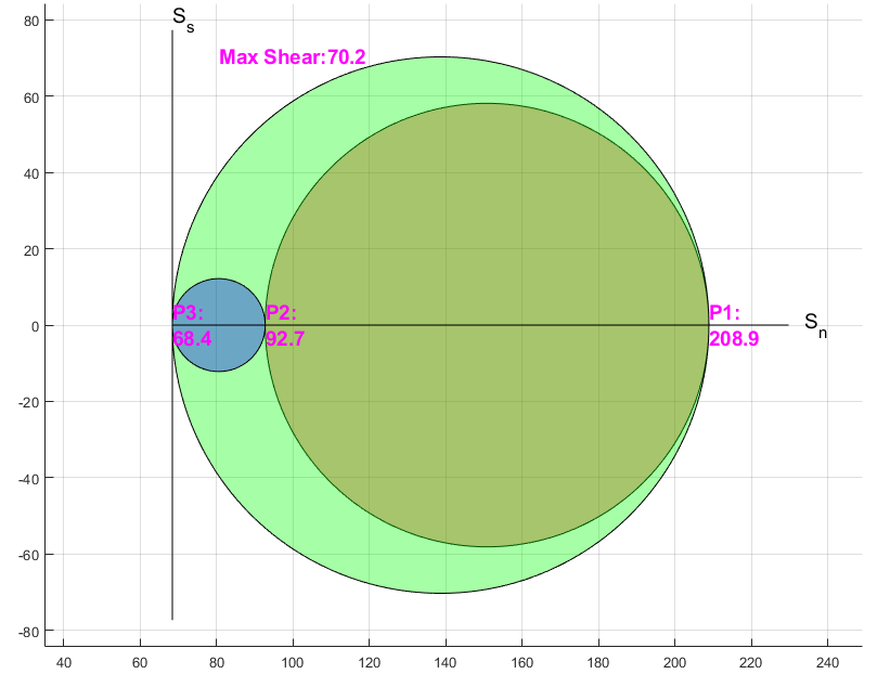
Construct the Mohr’s circle based on the calculated principal stresses. According to the diagram, the maximum shear stress is predicted to be 70.2 MPa. This value can also be computed using the following equation: \[\tau_{\text{max}} = \frac{|\sigma_1 - \sigma_3|}{2}\] Code: Plot Mohr's Circle
%plot mohrs circle---------------------------------------------------------
p12 = nsidedpoly(1000,'Center',[0.5*(Prin_Stress(1,1)+Prin_Stress(2,2))...
    0], 'Radius', 0.5*abs(Prin_Stress(1,1)-Prin_Stress(2,2)));
p13 = nsidedpoly(1000,'Center',[0.5*(Prin_Stress(1,1)+Prin_Stress(3,3))...
    0], 'Radius', 0.5*abs(Prin_Stress(1,1)-Prin_Stress(3,3)));
p23 = nsidedpoly(1000,'Center',[0.5*(Prin_Stress(2,2)+Prin_Stress(3,3))...
    0], 'Radius', 0.5*abs(Prin_Stress(2,2)-Prin_Stress(3,3)));
f2=figure;
figure(f2)
plot(p12, 'FaceColor', 'r')
hold on
plot(p13, 'FaceColor', 'g')
plot(p23, 'FaceColor', 'b')
grid on
text(Prin_Stress(1,1),0,['P1:' newline num2str(round(Prin_Stress(1,1),1))],...
'FontSize',14,'color','m','FontWeight','bold')
text(Prin_Stress(2,2),0,['P2:' newline num2str(round(Prin_Stress(2,2),1))],...
'FontSize',14,'color','m','FontWeight','bold')
text(Prin_Stress(3,3),0,['P3:' newline num2str(round(Prin_Stress(3,3),1))],...
'FontSize',14,'color','m','FontWeight','bold')
text(0.5*(Prin_Stress(2,2)+Prin_Stress(3,3)),0.5*abs(Prin_Stress(1,1)-...
    Prin_Stress(3,3)),['Max Shear:' num2str(round(0.5*abs(Prin_Stress(1,1)-...
    Prin_Stress(3,3)),1))],'FontSize',14,'color','m','FontWeight','bold')
axis equal
plot([Prin_Stress(3,3) 1.1*Prin_Stress(1,1)],[0 0],'k')
text(1.12*Prin_Stress(1,1),0,'S_n','FontSize',14)
plot([Prin_Stress(3,3) Prin_Stress(3,3)],[-0.55*abs(Prin_Stress(1,1)-...
    Prin_Stress(3,3)) 0.55*abs(Prin_Stress(1,1)-Prin_Stress(3,3))],'k')
text(Prin_Stress(3,3),0.57*abs(Prin_Stress(1,1)-Prin_Stress(3,3)),...
    'S_s','FontSize',14)
%--------------------------------------------------------------------------
The following code can be used to enhance the visualization of the stress tensor and the cross-sectional plane. Code: Plot Unit Cube and Cross Section Plane
%draw a unit cube centered at coordinate origin----------------------------
%this part of the code is only for visualization---------------------------
cube_corners= [...
         -0.5   -0.5    -0.5;
         0.5   -0.5     -0.5;
         0.5    0.5     -0.5;
         -0.5   0.5     -0.5;
         -0.5   -0.5     0.5;
         0.5   -0.5      0.5;
         0.5    0.5      0.5;
         -0.5   0.5      0.5];
xc = cube_corners(:,1);
yc = cube_corners(:,2);
zc = cube_corners(:,3);
idx = [1 2 3 4 1; 5 6 7 8 5; 1 2 6 5 1; 4 3 7 8 4; 2 3 7 6 2;1 4 8 5 1]';
figure(f1)
patch(xc(idx),yc(idx),zc(idx),'r', 'facealpha', 0.1)
xlabel('X')
ylabel('Y')
zlabel('Z')
view(3)
grid on
axis equal
hold on
plot3([-1.15 1.15],[0 0],[0 0],"b","LineWidth",1.5)
plot3([0 0],[-1.15 1.15],[0 0],"b","LineWidth",1.5)
plot3([0 0],[0 0],[-1.15 1.15],"b","LineWidth",1.5)
txt = '\leftarrow sin(\pi) = 0';
text(1.25,0,0,'X','FontSize',14)
text(0,1.25,0,'Y','FontSize',14)
text(0,0,1.25,'Z','FontSize',14)
xlim([-2 2])
ylim([-2 2])
zlim([-2 2])
%--------------------------------------------------------------------------

%draw the unit normal of the cross section---------------------------------
plot3([0 n(1,1)],[0 n(2,1)],[0 n(3,1)],"-.r","LineWidth",3)
text(1.1*n(1,1),1.1*n(2,1),1.1*n(3,1),'n','FontSize',14,'color', 'r')
%--------------------------------------------------------------------------

%draw a plane normal to n and passing through origin (0,0,0)---------------
%a plane is a*x+b*y+c*z+d=0  >>>>[a,b,c] is the normal
if n(3,1)==0
    if n(1,1)==0
       [xx,zz]=ndgrid(-0.75:0.5:0.75,-0.75:0.5:0.75);%create a grid
        yy=0*xx;
    elseif n(2,1)==0
       [yy,zz]=ndgrid(-0.75:0.5:0.75,-0.75:0.5:0.75);%create a grid
        xx=0*yy;
    else
       [yy,zz]=ndgrid(-0.75:0.5:0.75,-0.75:0.5:0.75);%create a grid
        xx=(-n(2,1)/n(1,1))*yy;
    end
else
    [xx,yy]=ndgrid(-0.75:0.5:0.75,-0.75:0.5:0.75);%create a grid
    zz=(-1/n(3,1))*(n(1,1)*xx+n(2,1)*yy);
end
surf(xx,yy,zz,'FaceAlpha',0.5,'EdgeColor', 'none', 'FaceColor', 'g')
%--------------------------------------------------------------------------
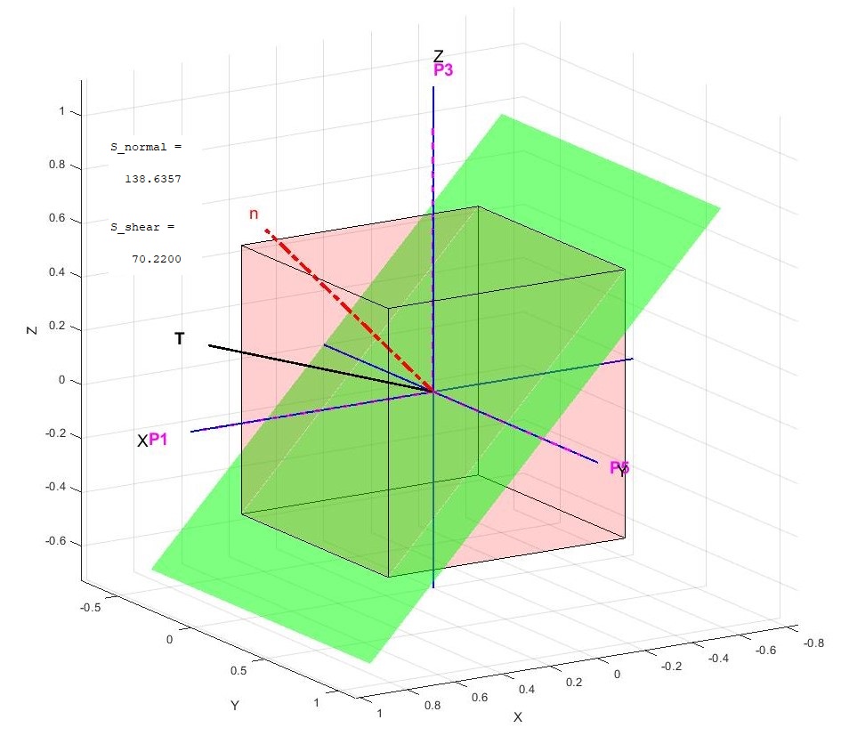
The same result can be obtained by calculating the shear and normal stresses in the eigenbasis, specifically along a direction 45 degrees from the second principal direction, defined as {1,0,1}. Code: Update Inputs
%INPUTS....................................................................
%S=[100 50 30; 50 150 40; 30 40 120];           %tensor in standard basis
S=[208.8557 0 0; 0 92.7286  0; 0 0 68.4157];    %tensor in principal basis
n=[1 0 1]';
%..........................................................................
\[[\sigma] = \begin{bmatrix} 208.8 & 0 & 0 \\ 0 & 92.7 & 0 \\ 0 & 0 & 68.4 \end{bmatrix}\]
The resulting plot is shown below. Note that in this case, the principal directions are aligned with the coordinate axes, as the stress tensor has been transformed into the eigenbasis.
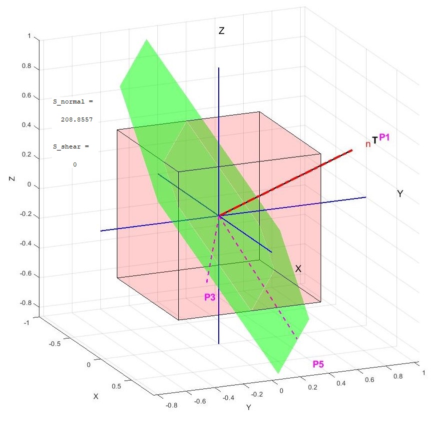
You are encouraged to modify the normal direction inputs and re-run the code to observe how the normal and shear stresses vary. For example, if the traction vector is calculated along a unit direction such as {0.4718 ,0.7334, 0.4894} in the standard basis, the shear stress on the plane would be zero, and the traction vector {T} would be aligned with the surface normal. Code: Update Inputs
%INPUTS....................................................................
S=[100 50 30; 50 150 40; 30 40 120];             %tensor in standard basis
%S=[208.8557 0 0; 0 92.7286  0; 0 0 68.4157];    %tensor in principal basis
n=[0.4718 0.7334 0.4894]';
%..........................................................................
The output of the code would be: